Slip distribution for different smoothing factors: (a) κ = 0 . 10, (b)

Download scientific diagram | Slip distribution for different smoothing factors: (a) κ = 0 . 10, (b) κ = 0 . 18, (c) κ = 0 . 30. We pick the second as the resultant model because of its good compatibility between weighted mis fi t and solution roughness. The numbers between the triangles in (a) indicate the segments. The white star denotes the epicenter from Harvard CMT solution.  from publication: 3-D coseismic displacement field of the 2005 Kashmir earthquake inferred from satellite radar imagery | Imagery, Imagery (Psychotherapy) and Earthquake | ResearchGate, the professional network for scientists.

a) Slip distribution (model A) of the 2011 Burma earthquake from both

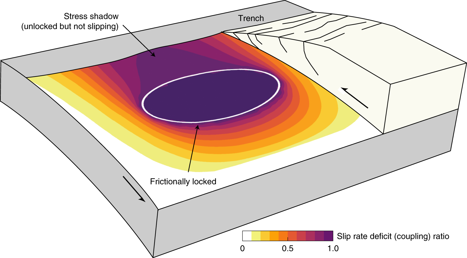
Slip rate deficit and earthquake potential on shallow megathrusts

Coseismic fault-slip distribution of the 2019 Ridgecrest Mw6.4 and Mw7.1 earthquakes

PDF) 3-D coseismic displacement field of the 2005 Kashmir earthquake inferred from satellite radar imagery

B-value variations in the Central Chile seismic gap assessed by a Bayesian transdimensional approach

Aseismic slip and recent ruptures of persistent asperities along the Alaska-Aleutian subduction zone

Models of distributed dip-slip along the subduction interface projected

Earthquake source region, stations, and slip distribution. (a) Map of

Improvement on spatial resolution of a coseismic slip distribution using postseismic geodetic data through a viscoelastic inversion, Earth, Planets and Space

A new method of variational Bayesian slip distribution inversion

PDF) 3-D coseismic displacement field of the 2005 Kashmir earthquake inferred from satellite radar imagery

Slip distribution for different smoothing factors: (a) κ = 0 . 10, (b)

Inversion of fault geometry and slip distribution of the 2017 Sarpol‐e